The Joule–Thomson effect

In 1853 Joule and William Thomson (in later life Lord Kelvin) did an experiment similar to the Joule experiment but allowing far more accurate results to be obtained.

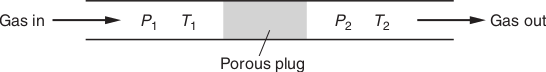
The Joule–Thomson experiment involves the slow throttling of a gas through a rigid, porous plug. An idealized sketch of the experiment is shown in Fig. 1.0. The system is enclosed in adiabatic walls, imposing the constraint of constant enthalpy, so that the process is isenthalpic. The left piston is held at a fixed pressure P₁. The right piston is held at a fixed pressure P₂ < P₁. The partition B is porous but not greatly so. This allows the gas to be slowly forced from one chamber to the other. Because the throttling process is slow, pressure equilibrium is maintained in each chamber. Essentially all the pressure drop from P₁ to P₂ occurs in the porous plug. In general there is a change in temperature (T₁ ≠ T₂) whenever the gas is real. Measurement of the temperature change ΔT = T₂ - T₁ in the Joule–Thomson experiment gives ΔT/ΔP at constant H. We define the Joule–Thomson coefficient, μ by

$${\mu }_{JT}\equiv {\left(\frac{\partial T}{\partial P}\right)}_H$$

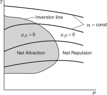
Real gases have nonzero Joule–Thomson coefficients. Depending on the identity of the gas, the pressure, the relative magnitudes of the attractive and repulsive intermolecular forces (see Molecular interpretation 2.1), and the temperature, the sign of the coefficient may be either positive or negative (Fig. 1.1). A positive sign implies that dT is negative when dP is negative, in which case the gas cools on expansion. In the case of real gases, μ is itself a function of temperature and pressure and is only positive in certain ranges of these variables. Gases that show a heating effect (μ_JT < 0) at one temperature show a cooling effect (μ_JT > 0) when the temperature is below their upper inversion temperature, T_I. A gas typically has two inversion temperatures, one at high temperature and the other at low.

In a gas expansion the pressure decreases, so the sign of ∂P is negative by definition. With that in mind: If the gas temperature is below the inversion temperature it cools if it is above the inversion temperature it warms up.

Helium and hydrogen are two gases whose Joule–Thomson inversion temperatures at a pressure of one atmosphere are very low (e.g., about 45 K (−228 °C) for helium). Thus, helium and hydrogen warm when expanded at constant enthalpy at typical room temperatures. On the other hand, nitrogen and oxygen, the two most abundant gases in air, have inversion temperatures of 621 K (348 °C) and 764 K (491 °C) respectively: these gases can be cooled from room temperature by the Joule–Thomson effect.

Figure 1.1 plots characteristic lines of constant enthalpy (isenthalps) on a T-P diagram. In the shaded region, the slopes of the curves are positive; therefore, μ_JT > 0. In this region, the temperature will decrease as the pressure decreases during the throttling process. Since the decrease in temperature as the pressure drops corresponds to a decrease in molecular kinetic energy, the molecular potential energy must be increasing or else energy conservation would be violated. We can say the molecules are more stable when they are closer together at the higher pressure and, consequently, that attractive forces are dominant in this region. Conversely, in the nonshaded region, the slopes of the isenthalps are negative; therefore μ_JT < 0. The temperature will increase as pressure decreases, indicating that repulsive forces dominate the behavior in this region. These two regions are separated by the inversion line, where the slope of T vs. P is zero and where attractive and repulsive interactions exactly balance. For a given pressure, the temperature at which these interactions balance is known as the Boyle temperature.

We want to calculate w, the work done on the gas in throttling it through the plug. The overall process is irreversible since P₁ exceeds P₂ by a finite amount, and an infinitesimal change in pressures cannot reverse the process. However, the pressure drop occurs almost completely in the plug. The plug is rigid, and the gas does no work on the plug, or vice versa. The exchange of work between system and surroundings occurs solely at the two pistons. Since pressure equilibrium is maintained at each piston, we can use dw_rev = PdV to calculate the work at each piston.

The Joule-Thomson experiment must be carefully distinguished from the adiabatic expansion of a gas in a piston and cylinder. The latter process normally leads to a cooling, on account of the decrease in internal energy consequent on the performance of work. On the other hand, the Joule-Thomson effect gives rise to a cooling only when μ_JT is positive.

Because all changes to the gas occur adiabatically, q = 0, which implies ∆U = w Consider the work done as the gas passes through the barrier. We focus on the passage of a fixed amount of gas from the high pressure side, where the pressure is P_i, the temperature T_i, and the gas occupies a volume V_i. The gas emerges on the low pressure side, where the same amount of gas has a pressure P_f, a temperature T_f , and occupies a volume V_f. The gas on the left is compressed isothermally by the upstream gas acting as a piston. The relevant pressure is P_i and the volume changes from V_i to 0; therefore, the work done on the gas is

The gas expands isothermally on the right of the barrier (but possibly at a different constant temperature) against the pressure P_f provided by the downstream gas acting as a piston to be driven out. The volume changes from 0 to V_f , so the work done on the gas in this stage is

The total work done on the gas is the sum of these two quantities, or

It follows that the change of internal energy of the gas as it moves adiabatically from one side of the barrier to the other is

Reorganization of this expression gives

or

An isenthalpic process.

Measurament of μ

The modern method of measuring μ_JT is indirect, and involves measuring the isothermal Joule–Thomson coefficient, the quantity

$${\mu }_T\equiv {\left(\frac{\partial H}{\partial P}\right)}_T$$

which is the slope of a plot of enthalpy against pressure at constant temperature. The first step in obtaining these results is to note that the Joule–Thomson coefficient involves the three variables T, P, and H. A useful result is immediately obtained by applying the Triple Product rule; in terms of these three variables that rule may be written:

$${\left(\frac{\partial T}{\partial P}\right)}_H{\left(\frac{\partial H}{\partial T}\right)}_P{\left(\frac{\partial P}{\partial H}\right)}_T=-1$$

it results that

To measure μ_T, the gas is pumped continuously at a steady pressure through a heat exchanger (which brings it to the required temperature), and then through a porous plug inside a thermally insulated container. The steep pressure drop is measured, and the cooling effect is exactly offset by an electric heater placed immediately after the plug (Fig. 2.30). The energy provided by the heater is monitored. Because the energy transferred as heat can be identified with the value of ∆H for the gas (because ∆H = q_p), and the pressure change ∆p is known, we can find μ_T from the limiting value of ∆H/∆p as ∆p → 0, and then convert it to μ. Table 2.9 lists some values obtained in this way

Molecular interpretation

An ideal gas becomes neither cooler nor warmer when passing through an expansion valve because there is no interaction, neither attractive nor repulsive, between ideal gas molecules, for an ideal gas, μ_JT is always equal to zero: ideal gases neither warm nor cool upon being expanded at constant enthalpy. But all real gases can interact. If the net interaction between gas molecules is attractive, increasing the distance between the molecules upon the expansion of the gas through the valve costs energy. Since this energy must come from the gas itself, cooling results. If the net interaction between gas molecules is repulsive, increasing the distance between the molecules upon the expansion of the gas through the valve yields energy. So warming results. At low temperatures, attractive interactions dominate because the gas molecules are moving slowly enough to be somewhat bonded to each other. At high temperatures gas molecules move too fast to notice any tendency to bond, so repulsion dominates. The cooling effect, which corresponds to μ > 0, is observed under conditions when attractive interactions are dominant (Z < 1), because the molecules have to climb apart against the attractive force in order for them to travel more slowly. For molecules under conditions when repulsions are dominant (Z > 1), the Joule–Thomson effect results in the gas becoming warmer, or μ < 0.

Linde refrigerator

The ‘Linde refrigerator’ makes use of Joule–Thompson expansion to liquefy gases (Fig. 2.33). The gas at high pressure is allowed to expand through a throttle; it cools and is circulated past the incoming gas. That gas is cooled, and its subsequent expansion cools it still further. There comes a stage when the circulating gas becomes so cold that it condenses to a liquid. For a perfect gas, μ = 0; hence, the temperature of a perfect gas is unchanged by Joule–Thomson expansion. This characteristic points clearly to the involvement of intermolecular forces in determining the size of the effect. However, the Joule–Thomson coefficient of a real gas does not necessarily approach zero as the pressure is reduced even though the equation of state of the gas approaches that of a perfect gas. The coefficient depends on derivatives and not on p, V, and T themselves.

«D- and L- configuration Index Internal Accusative»