The Dual Space
As we have studied, given two vector spaces V and W over 𝔽, the set of all linear maps V → W is a vector space denoted by Hom(V, W). A special case arises when W = 𝔽. The linear maps V → 𝔽 are called linear forms (or linear functionals) and they form a vector space V* = Hom(V, 𝔽), called the dual vector space, which is naturally associated to V. It turns out that a vector space V and its dual V* have the same dimension and are, hence, isomorphic.
Definition 7.2.1. Let V be a vector space over a field 𝔽. Then the dual of V, denoted by V*, is the vector space consisting of all linear forms on V.
V∗ := {linear functions f: V → 𝔽} □
Example 7.2.2. (Linear functionals on coordinate vector spaces) For the vector space 𝔽n (seen as a vector space of columns) the dual vector space (𝔽n)* = Hom(𝔽n, 𝔽) = M1,n (𝔽) consists of 1 × n matrices, that is, of row vectors, with entries in 𝔽. For such a row vector φ = (φ1, ..., φn) the action on a vector v ∈ V is given by matrix multiplication, so
φ(v) = φv = ∑ni=1 φivi (7.2.1)
Note that the matrix product of an 1 × n matrix (a row vector) with an n × 1 matrix (a column vector) is indeed a 1 × 1 matrix, so a number, as required. The expression on the right-hand side of Eq. (7.2.1) is, effectively, a dot product which we have now written as a matrix product.
To summarize, the elements of 𝔽n, as per our convention, can be viewed as column vectors while the elements of the dual, (𝔽n)*, can be viewed as row vectors, each with n entries in 𝔽. In particular, 𝔽n and (𝔽n)* have the same dimension. □
In the previous example we have seen that 𝔽n and its dual, (𝔽n)* have the same dimension. In fact, Theorem 3.4.2 proofs that dim𝔽 (V) = dim𝔽 (V*) is generally true. The following theorem provides another proof of this fact which relies on constructing the dual basis.
The Duality Principle
The condition of duality between two vector spaces is defined by the following.
Definition 7.2.2. Let {e1, e2, ..., en} be a basis in V and {e1, ..., en} a basis in V*. The two bases are said to be dual if
ei (ej) = δij
or using brackets as:
⟨ei | ej⟩ = δij
where δji is Kronecker's delta. □
The vectors in V are said to be contravariant, those in V*, covariant.
| Expansion of A | Projections | Component names |
|---|---|---|
| A = Σμ Aμ eμ | Aμ = A · eμ | Contravariant components of A |
| A = Σμ Aμ eμ | Aμ = A · eμ | Covariant components of A |
If {e1, e2, ..., en} be a basis in V, and f is a linear function on V, then ⟨f | ej⟩ = f(ej) give the numbers aj which determine the linear function f ∈ V* (cf. formula (7.2.2)). This remark implies that, if {e1, e2, ..., en} is a basis in V, then there exists a unique basis {f1, f2, ..., fn} in V* dual to {e1, e2, ..., en}. The proof is immediate
⟨f1 | e1⟩ = 1, ⟨f1 | e2⟩ = 0, ..., ⟨f1 | en⟩ = 0
define a unique vector (linear function) f1 ∈ V*. The equations
⟨f2 | e1⟩ = 0, ⟨f2 | e2⟩ = 1, ..., ⟨f2 | en⟩ = 0
define a unique vector (linear function) f2 ∈ V*, etc. The vectors f1, ..., fn are linarly independent since the corresponding n-tuples of numbers are linearly independent. Thus {f1, f2, ..., fn} costitute a unique basis of V* dual to the basis {e1, e2, ..., en} of V.
For example if V is ℝ2 choosing the canonical base {e1 = (1, 0), e2 = (0, 1)}, then e1 and e2 are linear forms such that e1(e1) = 1, e1(e2) = 0, e2(e1) = 0, and e2(e2) = 1.
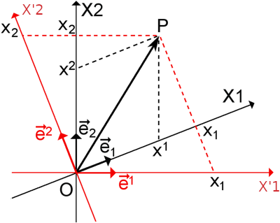
Figure 1 represents two coordinate systems where the contravariant and covariant components of OP are shown. The covariant components of OP appear in the axes of the two coordinate systems {X1; X2} and {X'1; X'2}. If we increase the length of a basis vector ej, we must decrease the contravariant component xj of OP in order to keep the latter unchanged. In other words, contravariant component xj transforms in the opposite way to basis vector ej. As a result, the dual basis vector ej decreases in length due to
ej ⋅ ej = ||ej|| ||ej|| cos θ = 1.
Therefore, the covariant component xj of OP in the dual coordinate system must increase in order to keep OP unchanged. In other words, covariant components xj in the dual coordinate system transforms in the same way as basis vector ej.
Example 7.2.3. The gradient F(x) of ∇F: V ⟶ ℝ at any point x ∈ V is in the dual space V* of (continuous) linear functionals on V. ■
Dirac’s Bracket Notation
To emphasize the duality between the two vector spaces, one takes advantage of Dirac’s bra-ket notation, which he originally introduced into quantum mechanics.
If f is a linear function on V and f(v) is its value at v ∈ V, then one also write
f(v) ≡ ⟨f|v⟩ ≡ ⟨f̲|v⟩
Thus the underscore under f is a reminder that f̲ ∈ V∗, while v, or better v is an element of V. We say that f operates on the vector v and produces
⟨f|v⟩
A covector can thus be thought as an operator which acts on a vector and outputs a number.
Let e1, e2, ..., en be a basis in an n-dimensional space V. If
x = ξ1e1 + ξ2e2 + ... + ξnen
is a vector in V and f is a linear function on V, then we can write
f(x) = f(ξ1e1 + ξ2e2 + ... + ξnen)
= a1 ξ1 + a2 ξ2 + ... + an ξn 7.2.1
where the coefficients a1, a2, ..., an which determine the linear function are given by
a1 = f(e1), a2 = f(e1), ..., an = f(en) 7.2.2
It is clear from Eq. 7.2.1 that given a basis, e1, e2, ..., en every n-tuple a1, a2, ..., an determines a unique linear function. Further since this correspondence with a1, a2, ..., an preserves sums and products (of vectors by scalars), it follows that V* is isomorphic to the space of n-tuples of numbers. One consequence of this fact is that the dual space i of the n-dimensional space V is likewise n-dimensional.
Double Dual space V**
The isomorphism between V and V∗ depends on the particular choice of basis that we make on V—if we change the basis B in Theorem 7.1.4 then the vector v corresponding to a linear form f changes as well; we call such an isomorphism non-canonical. The fact that the isomorphism between V and V∗ is basis-dependent suggests that something somewhat unnatural is going on, as many (even finite-dimensional) vector spaces do not have a “natural” or “standard” choice of basis. However, if we go one step further and consider the double-dual space V∗∗ consisting of linear forms acting on V∗ then we can find an isomorphism between V and V∗* which is basis independent. So we now briefly explore this double-dual space.
The members of V∗∗ are linear forms acting on linear forms (i.e., functions of functions).
Using the exact same ideas as earlier, if V is finite-dimensional then we still have dim(V∗∗) = dim(V∗) = dim(V), so all three of these vector spaces are isomorphic. Consider the function T: V ⟶ V** defined by
T(v) = φv 7.2.3
with v ∈ V and φv ∈ V**. T is a function that sends vectors to functions of functions of vectors. The linear form φv ∈ V∗∗ in 7.2.3 is defined by
φv(f) = f(v) for all f ∈ V∗ 7.2.4
Showing that φv is linear form does not requires just to check the two defining properties from the Definition of linear forms:
For all f , g ∈ V∗ we have
φv(f + g) = (f + g)(v) = f(v) + g(v) = φv(f) + φv(g).
Similarly, for all c ∈ 𝕂 and f ∈ V∗ we have
φv(cf) = (cf)(v) = cf(v) = cφv(f)
To prove that T is a canonical isomorphism we need the following Lemma.
Lemma 7.2.4. Let T: V → V** the canonical double-dual isomorphism defined as eq. 7.2.3. If B = {v1, v2, ..., vn} ⊆ V is linearly independent then so is B' = {T(v1), T(v2), ..., T (vn)}⊆ V**.
Proof. Suppose that
c1T (v1) ··· + cnT (vn) = 0.
By linearity of T, this implies T (c1 v1 + ··· + cn vn) = 0, so φc1 v1 + ··· + cn vn = 0, which implies
φc1 v1 + ··· + cn vn(f) = f(c1 v1 + ··· + cn vn) = c1 f(v1) + ··· + cn f(vn) = 0
for all f ∈ V*.
Theorem 7.2.5. The function T: V → V** defined by T (v) = φv where φv ∈ V** is defined as Equation 7.2.4, is an isomorphism.
Proof. We must show that T is linear and invertible. Before showing that T is linear, we first make a brief note on notation. Since T maps into V∗∗, we know that T(v) is a function acting on V*. We thus use the notation T (v)(f) or to refer to the scalar value that results from applying the function T(v) to f ∈ V*. For linearity, for all f ∈ V* we have
T (v + w)(f) = φv + w(f) (definition of T)
= f(v + w) (definition of φv + w)
= f (v) + f(w) (linearity of each f ∈ V*)
= φv (f) + φw (f) (definition of φv and φw)
= T (v)(f) + T(w)(f). (definition of T)
and
T (cv)(f) = φcv(f) = f (cv) = cf(v) = cφv(f) = cT(v)(f)
for all f ∈ V*, so T (cv) = cT(v) for all c ∈ 𝕂.
For invertibility, we claim that if B = {v1, v2, ..., vn} is linearly independent then so is B' = {T(v1), T(v2), ..., T (vn)} (this claim is pinned down in Exercise 1.3.24). Since B' contains n = dim(V) = dim(V**) vectors, it must be a basis of V** by Exercise 1.2.27(a). It follows that [T]B'←B = I, which is invertible, so T is invertible as well. □